Shaun D Jackman, Anthony G Raymond and İnanç Birol
Canada’s Michael Smith Genome Sciences Centre
The development of long-distance genome sequencing libraries, known as mate-pair or jumping libraries, allows the contigs of a de novo genome sequence assembly to be assembled into scaffolds, which specify the order and orientation of those contigs. We have developed for the de novo genome sequence assembly software ABySS a series of heuristic algorithms, each of which identifies a small subgraph of the scaffold graph matching a particular topology and applies a transformation to that subgraph to simplify the scaffold graph. These algorithms eliminate ambiguities in the scaffold graph and identify contigs that may be assembled into a scaffold.
Modern short read genome sequencing technology produces billions of short read, each 150 base pairs in length, although this length is continually increasing. When a reference genome sequence is available, these reads may be aligned to that reference to identify single nucleotide variants, other small sequence variants and large structural variation. When a reference sequence is not available, or when the experiment wishes to avoid being biased by the reference sequence, the sequence reads must be assembled de novo. Due to gaps in the sequencing and repetitive genome sequence, such an assembly is often fragmented into many sequences, called contigs. The relative order and orientation of these contigs is unknown, and the challenge of ordering and orienting these contigs is called scaffolding.
Scaffolding is accomplished using paired-end sequencing, where both ends of the same DNA fragment are sequenced. The success of scaffolding is limited by the size of the fragment library and its ability to span the largest repeat sequences of the genome. Until recently, a paired-end sequencing library was limited to approximately 800 base pairs. New techniques in library construction have allowed for the construction of mate-pair libraries as large as 5000 bp. New sequencing technologies require the development of new algorithms to fully exploit the technology. Further developing our work on the de novo sequencing assembly software, ABySS, we have developed a novel scaffolding algorithm capable of scaffolding very large genomes. We have used ABySS to scaffold the genome sequence assembly of the white spruce tree, Picea glauca, whose 20 gigabase genome is roughly seven times the size of the human genome.
A scaffold graph is composed of vertices representing sequences and edges representing a bundle of paired-end reads, which indicate an order and orientation of those two contigs as well as a rough estimate of the distance separating the two sequences. Our scaffolding algorithm is implemented as a series of heuristic graph transformations, each of which identifies a small subgraph matching a topology typical of a particular genomic feature, such as a repeat sequence, and applies a transformation to that subgraph to successively simplify the scaffold graph. These algorithms eliminate ambiguities in the scaffold graph and identify contigs that are assembled into scaffolds.
We compare our scaffolding results to that of the de novo assembly software packages ALLPATHS-LG, SGA and SOAPdenovo. These three software packages and ABySS were used to assemble short-read sequencing data of the human sample NA12878. The scaffolds of these assemblies were aligned to the reference human genome to determine the contiguity and correctness of the scaffolds and compare the performance of these tools.
A scaffold graph is a directed graph where each vertex represents a contig sequence. Each directed edge e = (u,v) represents a bundle of paired reads joining two contigs, where, for each pair, one read aligns to the sequence of vertex u and the other read aligns to the sequence of vertex v. The direction of the edge (u,v) indicates that the orientation of the reads show that contig v occurs after the contig u in the genome.
A scaffold graph is a skew-symmetric graph. Every vertex u has a complementary vertex ~u whose sequence is the reverse complement of the sequence of vertex u. Every edge (u,v) has a complementary edge (~v,~u). Any graph manipulation operations maintain this property.
Properties are associated with each vertex, such as the length of the sequence, and each edge, such as the number of paired reads supporting the edge.
The property g[e].n, where e = (u,v), is the number of paired reads where one read maps to the sequence of vertex u and the second read maps to the sequence of vertex v with orientations that agree with the direction of the edge e.
The following graph-manipulation procedures are used to define algorithms.
The scaffolding algorithm is implemented as a sequence of heuristics that each identify subgraphs that match a particular topology and then transform that subgraph in some by way by adding and removing vertices and edges. Although not shown explicitly in the algorithms below, for each algorithm the modifications of the graph decided by that algorithm are performed simultaneously, so that the result does not depend on the order in which the vertices and edges are visited by the traversal of the graph.
Short contigs and edges that are poorly supported by paired reads are removed from the graph. Vertices shorter than s bp are removed from the graph, and edges supported by fewer than n paired reads are removed from the graph, where s and n are parameters of the algorithm. Short contigs may be repetitive, and poorly supported edges may result from reads that are incorrectly mapped to the assembly.
procedure filter_graph(graph g):
for vertex u in g
    if g[u].l < s
        remove_vertex(u, g)
for edge e in g
    if g[e].n < n
        remove_edge(e, g)
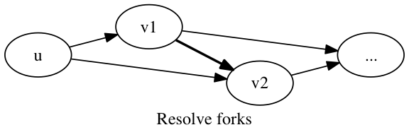
A fork is composed of two edges (u,v1) and (u,v2) with no edge (v1,v2) or (v2,v1) present in the graph g. The vertices v1 and v2 are known to follow u, but it is unknown whether v1 follows v2 or vice versa. There may exist an edge in the original graph g0, prior to filtering, that resolves this ambiguity of the relative order of v1 and v2. We check whether the edges (v1,v2) and (v2,v1) exist in the graph g0, and if precisely one such edge exists, we add it to the graph g.
procedure resolve_forks(graph g0, graph g):
for edges (u,v1), (u,v2) in g
    if exists (v1,v2) in g0 and not exists (v2,v1) in g0
        add_edge(v1, v2, g)
    if exists (v2,v1) in g0 and not exists (v1,v2) in g0
        add_edge(v2, v1, g)
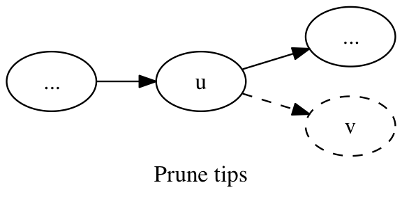
A tip is a vertex that forms a short spur extending from an otherwise contiguous path. It has in-degree = 1 and out-degree = 0. These tips are removed from the graph.
procedure prune_tips(graph g):
for edge (u,v) in g
    if g[u].outdeg > 1 and g[v].indeg = 1 and g[v].outdeg = 0
        remove_vertex(v, g)
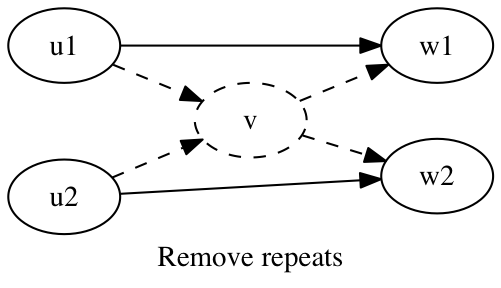
A repeat is a sequence that occurs multiple times in the genome being assembled. A repeat that is small enough to be spanned by paired reads causes telltale transitive edges in the scaffold graph. These transitive edges will eventually be removed from the scaffold graph, but removing these transitive edges from the scaffold graph removes the very information that would resolve the repeat. Before removing transitive edges, we identify and remove vertices caused by repetitive sequence.
procedure remove_repeats(graph g):
for edges (u1,w1), (u2,w2), (u1,v), (v,w1), (u2,v), (v,w2) in g
    remove_vertex(v, g)
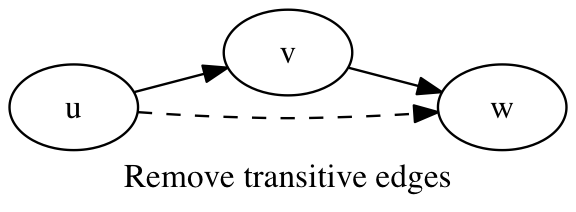
An edge (u,w) is transitive if there exists a path in the graph from vertex u to vertex w. Finding and removing all transitive edges from a graph is a potentially time-consuming operation. We can however easily find the transitive edges with a maximum path length of two, which are removed from the graph.
procedure remove_transitive_edges(graph g):
for edges (u,v), (v,w), e = (u,w) in g
    remove_edge(e, g)
A bubble in a graph is defined by Heng Li as follows:
A bubble is a directed acyclic subgraph with a single source and a single sink having at least two paths between the source and the sink. A closed bubble is a bubble with no incomming edges from or outgoing edges to other parts of the entire graph, except at the source and the sink vertices. A closed bubble is simple if there are exactly two paths between the source and the sink; otherwise it is complex.
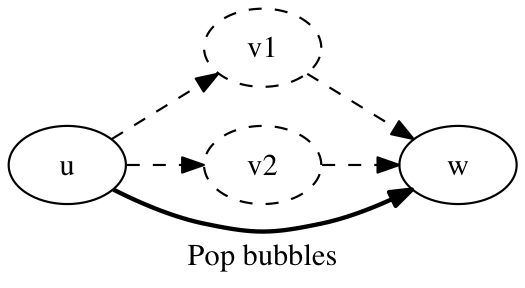
A missing edge in the scaffold graph, due to a lack of coverage, typically results in a simple closed bubble, where two vertices, v1 and v2, are known to occur between two other vertices, u and w, but the lack of an edge between v1 and v2 means the order of v1 and v2 is unknown. This situation is resolved by removing the vertices v1 and v2 from the graph and adding the edge (u,w).
procedure remove_simple_bubbles(graph g):
for edges (u,v1), (v1,w), (u,v2), (v2,w) in g
    remove_vertex(v1, g)
    remove_vertex(v2, g)
    add_edge(u, w, g)
Complex bubbles may be similarly identified and removed. A topological ordering of the graph is computed using a depth-first search (DFS). Back-edges that result from cycles in the graph are safely ignored, since bubbles are, by this definition, acyclic subgraphs. The topological ordering computed by the DFS groups the vertices of a closed bubble together in the topological ordering, and this property is used to identify and remove complex closed bubbles from the scaffold graph.
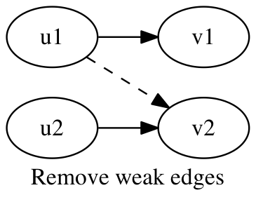
An edge e = (u1,v2) is defined as weak if there exists edges e1 = (u1,v1) and e2 = (u2,v2) in the graph where g[e].n < g[e1].n and g[e].n < g[e2].n. Weak edges may result from reads that are incorrectly mapped to the assembly. These weak edges are removed from the graph.
procedure remove_weak_edges(graph g):
for edges e = (u1,v2), e1 = (u1,v1), e2 = (u2,v2) in g
    if g[e].n < g[e1].n and g[e].n < g[e2].n
        remove_edge(e, g)
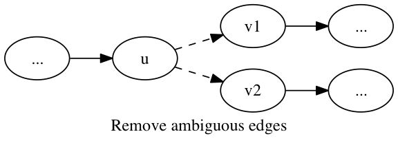
An edge (u,v) is ambiguous if either the out-degree of u or the in-degree of v is greater than one. These ambiguous edges are removed from the graph.
procedure remove_ambiguous_edges(graph g):
for edge e = (u, v) in g
    if g[u].outdeg > 1 or g[v].indeg > 1
        remove_edge(e, g)
The remaining edges form contiguous paths, which are assembled to create the final scaffolds. The sequences of the vertices in a path are concatenated, interspersed with gaps represented by a run of the character N, whose length corresponds to the estimate of the distance between those two contigs. A maximum likelihood estimator is used to estimate the distance between the two contigs from the alignments of the paired reads to the contigs. It is possible that the distance estimate is negative, indicating that the two contigs should in fact overlap. If such an overlap is indeed found in the contig overlap graph, the two contigs are merged.
We assembled the 101-bp paired-end sequencing data of the human
sample NA12878 using ABySS. Scaffolds were
split at N to obtain contigs. The contigs were aligned to the human
reference GRCh37 using BWA-SW with the command line bwa
bwasw -b9 -q16 -r1 -w500. Alignments at least 200 bp in length were
used to calculate the aligned contig N50, excluding secondary
alignments of a query that overlap a larger alignment by more than
50% of the smaller alignment. Alignments at least 500 bp in length
with a mapping quality of at least 10 were used to identify
breakpoints in the alignments of contigs to the reference.
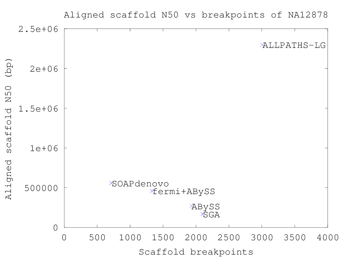
The position of the contigs in each scaffold were compared to the position of the contigs aligned to the reference genome to identify contigs that do not align in a manner that agrees with their arrangement in the scaffold. For a sequence of contigs in a scaffold, the start positions of those contigs on the reference genome must be a monotonically increasing sequence, or decreasing if the scaffold is reverse-complemented with respect to the reference, and likewise the end positions must also be a monotonically increasing sequence. The scaffold is broken at any pair of contigs that do not satisfy these criteria, and the aligned scaffold N50 is calculated.
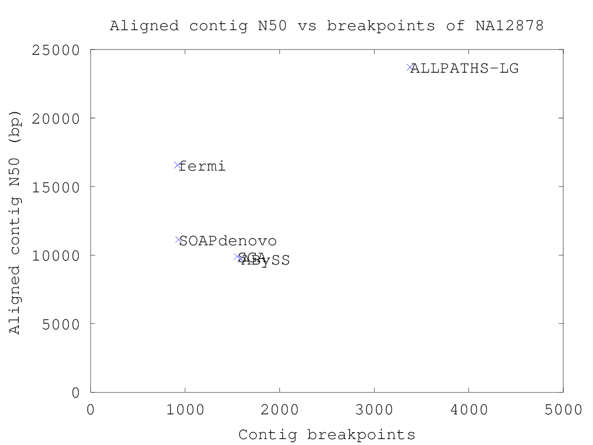
This analysis was repeated for assemblies of NA12878 by ALLPATHS-LG, fermi, SGA and SOAPdenovo. The ALLPATHS-LG assembly is downloaded from NCBI, and the fermi, SGA and SOAPdenovo assemblies were provided by Heng Li, Jared Simpson and Ruibang Luo respectively (see Materials). The ABySS, fermi, SGA and SOAPdenovo assemblies use identical data sets. The ALLPATHS-LG assembly uses a deeper 100x data set and two mate-pair libraries. The contigs assembled by fermi were assembled into scaffolds using the scaffolding algorithm of ABySS.
| ABySS | ALLPATHS-LG | fermi | SGA | SOAPdenovo | |
|---|---|---|---|---|---|
| Contig bp | 2.70 G | 2.61 G | 2.75 G | 2.76 G | 2.66 G |
| Aligned contig bp | 2.69 G | 2.61 G | 2.73 G | 2.74 G | 2.64 G |
| Covered ref. bp | 2.66 G | 2.59 G | 2.70 G | 2.70 G | 2.64 G |
| Contig N50 | 9.75 k | 23.8 k | 16.6 k | 9.91 k | 11.1 k |
| Aligned contig N50 | 9.72 k | 23.7 k | 16.6 k | 9.90 k | 11.1 k |
| Contig breakpoints | 1590 | 3380 | 920 | 1549 | 931 |
| Scaffold N50 | 273 k | 11.5 M | 446 k | 167 k | 565 k |
| At least 500 bp & Q10 | 276 k | 11.3 M | 462 k | 173 k | 565 k |
| Aligned scaffold N50 | 270 k | 2.30 M | 458 k | 168 k | 557 k |
| Scaffold breakpoints | 1933 | 3008 | 1333 | 2101 | 717 |
Plotting the aligned contig N50 versus the number of breakpoints yields a plot where the best assemblies are found in the top-left corner. Plotting the aligned scaffold N50 versus the number of scaffold breakpoints yields a similar plot showing the performance of the scaffolding algorithm.
The sequencing data of human sample NA12878 (SRS000090) is 101-bp Illumina reads.
Eight lanes of paired-end data were used, four lanes of the paired-end library Solexa–18483 and four lanes of the library Solexa–18484: ftp://hengli:reichdata@ftp.broadinstitute.org/NA12878-hs37d5-aln/NA12878-hs37.bam
| Library | Lane | Reads | Bases (bp) |
|---|---|---|---|
| Solexa–18483 | 20FUKAAXX100202_1 | 159875468 | 16.1 G |
| Solexa–18483 | 20FUKAAXX100202_3 | 154900876 | 15.6 G |
| Solexa–18483 | 20FUKAAXX100202_5 | 156932536 | 15.9 G |
| Solexa–18483 | 20FUKAAXX100202_7 | 155034158 | 15.9 G |
| Solexa–18484 | 20FUKAAXX100202_2 | 149658350 | 15.1 G |
| Solexa–18484 | 20FUKAAXX100202_4 | 145881464 | 14.7 G |
| Solexa–18484 | 20FUKAAXX100202_6 | 147970372 | 14.9 G |
| Solexa–18484 | 20FUKAAXX100202_8 | 150971682 | 15.2 G |
| Total | 1221224906 | 123.3 G |
Four lanes of the mate-pair library Solexa–30807 (SRX027699) were used: http://sra.dnanexus.com/experiments/SRX027699
| SRA run | Lane | Reads | Bases (bp) |
|---|---|---|---|
| SRR067773 | 2025JABXX100603_5 | 186100680 | 18.8 G |
| SRR067778 | 2025JABXX100603_7 | 194515894 | 19.6 G |
| SRR067779 | 2025JABXX100603_6 | 188012974 | 19.0 G |
| SRR067786 | 2025JABXX100603_8 | 189208654 | 19.1 G |
| Total | 757838202 | 76.5 G |
JT Simpson, K Wong, SD Jackman, JE Schein, SJM Jones, İ Birol (2009). ABySS: a parallel assembler for short read sequence data. Genome research, 19 (6), 1117–1123.
Gnerre S, MacCallum I, Przybylski D, Ribeiro F, Burton J, Walker B, Sharpe T, Hall G, Shea T, Sykes S, Berlin A, Aird D, Costello M, Daza R, Williams L, Nicol R, Gnirke A, Nusbaum C, Lander ES, Jaffe DB (2011). High-quality draft assemblies of mammalian genomes from massively parallel sequence data. Proceedings of the National Academy of Sciences, 108 (4), 1513–1518.
Li H. and Durbin R. (2010). Fast and accurate long-read alignment with Burrows-Wheeler Transform. Bioinformatics, Epub.
Mark A DePristo, Eric Banks, Ryan Poplin, Kiran V Garimella, Jared R Maguire, Christopher Hartl, Anthony A Philippakis, Guillermo del Angel, Manuel A Rivas, Matt Hanna, Aaron McKenna, Tim J Fennell, Andrew M Kernytsky, Andrey Y Sivachenko, Kristian Cibulskis, Stacey B Gabriel, David Altshuler and Mark J Daly (2011). A framework for variation discovery and genotyping using next-generation DNA sequencing data. Nature Genetics 43 (5), 491–498.
Heng Li (2012). Exploring single-sample SNP and INDEL calling with whole-genome de novo assembly. Bioinformatics, advance access.
Jared T Simpson and Richard Durbin (2012). Efficient de novo assembly of large genomes using compressed data structures. Genome Research, 22 (3), 549–556.
Ruiqiang Li, Hongmei Zhu, Jue Ruan, Wubin Qian, Xiaodong Fang, Zhongbin Shi, Yingrui Li, Shengting Li, Gao Shan, Karsten Kristiansen, Songgang Li, Huanming Yang, Jian Wang and Jun Wang (2010). De novo assembly of human genomes with massively parallel short read sequencing. Genome Research, 20 (2), 265–272.